If you have a problem or need to report a bug please email : support@dsprobotics.com
There are 3 sections to this support area:
DOWNLOADS: access to product manuals, support files and drivers
HELP & INFORMATION: tutorials and example files for learning or finding pre-made modules for your projects
USER FORUMS: meet with other users and exchange ideas, you can also get help and assistance here
NEW REGISTRATIONS - please contact us if you wish to register on the forum
Users are reminded of the forum rules they sign up to which prohibits any activity that violates any laws including posting material covered by copyright
Tweaked One pole LPF
Tweaked One pole LPF
![]() by juha_tp » Thu Mar 28, 2019 6:12 pm
by juha_tp » Thu Mar 28, 2019 6:12 pm
So, as winked, coefficients are calculated this way (Matlab/Octave code):
- Code: Select all
// fs - in Hz (tested only @  44100)
// fct - in µs, if Hz used then convert to µs with formula 1/(2*pi*fc)
x = 1.0/(fs*fct);
a0 = 1.0;
a1 = -(1 + x + 0.5 * x^2); // Taylor
b0 = a0 + a1;
b1 = 0.0;

a = [a0 a1];
b = [b0 b1];
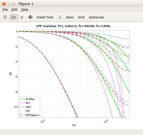
Comparison against MZT, IIM and BLT: https://i.postimg.cc/zDPyPrRz/lpf-robo.png (cut-offs: 1k, 5k, 10k, 15k, 20k)
I also did run speed comparison against the original exp() based filter implementation and got about 20x speed up with this tweak (Ubuntu, g++, --ffast-math enabled).
Octave code for the linked plot image:
- Code: Select all
% --------------------
% OCTAVE PACKAGES
% --------------------
pkg load signal
% --------------------

%clf

fs=44100;
fc=1000;
fct=1/(2*pi*fc);
fs2 = fs/2;
N=1; % order

% -----------------------------
% Analog model
% --------------------
w0 = 2*pi*fc;
Analogb = 1;
Analoga = [1 w0];
Analog = tf(Analogb, Analoga);
Analog = Analog/dcgain(Analog);

% --------------------
% MZT
% --------------------
p1 = exp(-1.0/(fs*(1/(2 * pi * fc))))
z1 = 0.0;
MZTa0 = 1.0;
MZTa1 = -p1;
MZTb0 = 1.0-p1;
MZTb1 = -z1;

MZTa = [MZTa0 MZTa1];
MZTb = [MZTb0 MZTb1];

MZT=tf(MZTb, MZTa, 1/fs);

% --------------------
% IIM
% --------------------

[IIMb,IIMa]=impinvar(Analogb,Analoga,fs);
IIM=tf(IIMb, IIMa, 1/fs);
IIM=IIM/dcgain(IIM);

% --------------------
% MZT approximated
% --------------------
x = 1.0/(fs*fct);
MZTa0 = 1.0;
MZTa1 = -(1 + x + 0.5 * x^2);
MZTb0 = MZTa0 + MZTa1;
MZTb1 = 0.0;

MZTa = [MZTa0 MZTa1];
MZTb = [MZTb0 MZTb1];

MZT2=tf(MZTb, MZTa, 1/fs);


% --------------------
% BLT
% --------------------
w0 = 2*pi*(fc/fs);
%BLTb0 =   sin(w0);
%BLTb1 =   sin(w0);
%BLTa0 =   cos(w0) + sin(w0) + 1.0;
%BLTa1 =   sin(w0) - cos(w0) - 1.0;
%
%BLTa = [BLTa0 BLTa1];
%BLTb = [BLTb0 BLTb1];
%
%BLT=tf(BLTb, BLTa, 1/fs);
%BLT=BLT/dcgain(BLT);

BLT = c2d(Analog, 1/fs, 'prewarp', w0);

% --------------------
% Plot
% --------------------

nf = logspace(0, 5, fs2);

figure(1);
% analog model
[mag, pha] = bode(Analog,2*pi*nf);
semilogx(nf, 20*log10(abs(mag)), 'color', 'g', 'linewidth', 2);
axis([10 fs2 -30 1]);
hold on;
%semilogx(nf, pha, 'color', 'g', 'linewidth', 2, 'linestyle', '--');

% BLT
[mag, pha] = bode(BLT,2*pi*nf);
semilogx(nf, 20*log10(abs(mag)), 'color', 'm', 'linewidth', 1.0, 'linestyle', '-');
%semilogx(nf, pha, 'color', 'm');

% MZT
[mag, pha] = bode(MZT,2*pi*nf);
semilogx(nf, 20*log10(abs(mag)), 'color', 'k', 'linewidth', 1.0, 'linestyle', '-');
%semilogx(nf, pha, 'color', 'k', 'linewidth', 1.0, 'linestyle', '--');

% IIM
[mag, pha] = bode(IIM,2*pi*nf);
semilogx(nf, 20*log10(abs(mag)), 'color', 'c', 'linewidth', 1.0, 'linestyle', '--');
%semilogx(nf, pha, 'color', 'c', 'linewidth', 1.0, 'linestyle', '--');

% MZT approximated
[mag, pha] = bode(MZT2,2*pi*nf);
semilogx(nf, 20*log10(abs(mag)), 'color', 'r', 'linewidth', 2.0, 'linestyle', '--');
%semilogx(nf, -pha, 'color', 'r', 'linewidth', 2.0, 'linestyle', '--');

grid on;

str=num2str(fs);
str2=num2str(fc);
str3=num2str(N);

str = sprintf("LPF (various TF), order:%s, fs=%s, fc=%s, ",str3, str, str2);
title(str);
legend('Analog', 'BLT', 'MZT', 'IIM', 'MZTapprox', 'location', 'southwest');
xlabel('Hz');ylabel('dB');
- juha_tp
- Posts: 57
- Joined: Fri Nov 09, 2018 10:37 pm
Re: Tweaked One pole LPF
![]() by wlangfor@uoguelph.ca » Fri Mar 29, 2019 9:15 pm
by wlangfor@uoguelph.ca » Fri Mar 29, 2019 9:15 pm
-

wlangfor@uoguelph.ca - Posts: 912
- Joined: Tue Apr 03, 2018 5:50 pm
- Location: North Bay, Ontario, Canada
Re: Tweaked One pole LPF
![]() by lalalandsynth » Wed Apr 03, 2019 12:06 am
by lalalandsynth » Wed Apr 03, 2019 12:06 am
-

lalalandsynth - Posts: 600
- Joined: Sat Oct 01, 2016 12:48 pm
Re: Tweaked One pole LPF
![]() by juha_tp » Wed Apr 03, 2019 8:23 am
by juha_tp » Wed Apr 03, 2019 8:23 am
lalalandsynth wrote:Is it possible to design filters in matlab and get code that works in FS DSP/assembler?
Nope, if you plan to use Matlab build in functions for to design the filters. IIRC, Matlab can export to c/c++ but my quess is that most Matlab related functions/code uses header and library files by Mathworks (licencing).
Compiler explorer probably could help in bringing the C -code to FS Assembler ... haven't checked it but, here's an example based on my post above.
- juha_tp
- Posts: 57
- Joined: Fri Nov 09, 2018 10:37 pm
Who is online
Users browsing this forum: No registered users and 7 guests